

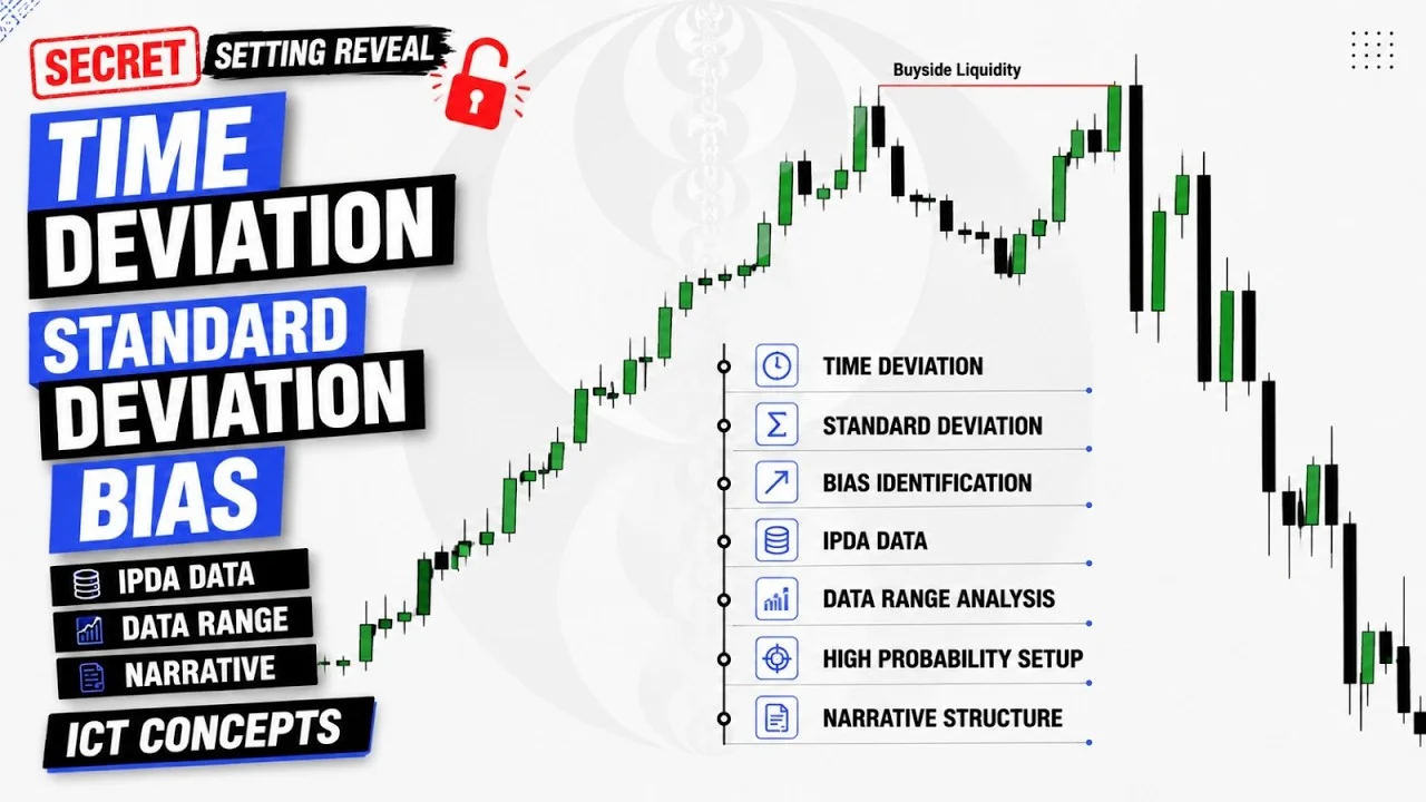
Standard Deviation, IPDA Ranges, and Time-Based Liquidity: A Complete Framework for Market Bias
This guide details the advanced application of Standard Deviation (SD), Interbank Price Delivery Algorithm (IPDA) data ranges, and time-based liquidity concepts. It moves beyond basic target projection to explain how institutions deliver price through specific manipulation and distribution legs. By aligning higher-timeframe candles with lower-timeframe structures, traders can identify precise reversal points, determine market bias before price movement occurs, and distinguish between internal retracements and external trend continuations. The framework relies on specific SD settings, body-closing confirmations, and a three-candle lookback period to predict whether a market will hunt a high or reverse immediately.
Introduction to Advanced Market Concepts▶ 0:00
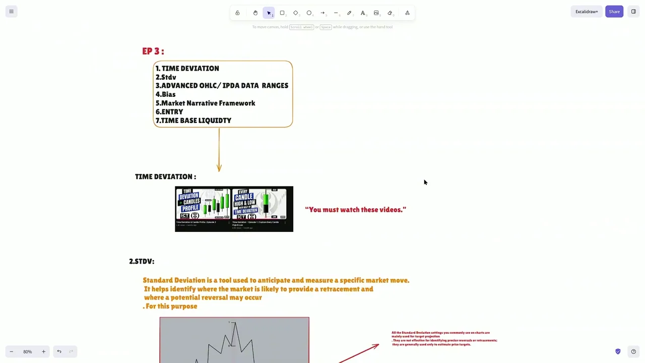
Most traders operate with a limited understanding of market mechanics, focusing primarily on basic liquidity sweeps or standard ICT concepts without grasping the underlying data delivery systems. This analysis covers topics that differentiate professional execution from retail guessing, specifically focusing on how markets deliver price in relation to time and specific algorithmic levels. The core subjects include Time Deviation, Standard Deviation (SD), Advanced OHLC/IPDA Data Ranges, Bias determination, Market Narrative Frameworks, Entry techniques, and Time-Based Liquidity.
While Time Deviation has been covered in previous discussions regarding how to capture the high and low of specific candles at specific times, this session focuses heavily on Standard Deviation and its true utility. Many existing resources misrepresent SD as merely a tool for projecting profit targets. In reality, when configured correctly, SD is a primary mechanism for identifying reversals, determining bias, and capturing both the high and low of a market move before it fully develops.
The methodology presented here requires a shift away from common SD settings found on social media platforms. Those standard settings are designed only for target estimation after a trade is already taken. The custom configuration detailed below allows for the identification of "hotspots" where price is algorithmically bound to react, providing sniper entries and clear invalidation points.
Understanding Standard Deviation and Common Misconceptions▶ 5:30
Standard Deviation is a tool used to measure a specific market move and anticipate where that move will terminate. In typical usage, traders plot an SD from a significant high to a low following a structure shift. This generates levels such as -1, -1.5, -2, -2.5, -3, -3.5, -4, and -4.5. Traders often mark broad zones around these levels, expecting price to reverse within them.
This approach is fundamentally flawed for entry purposes. If a trader identifies a zone at -1 or -1.5 but fails to consider that the algorithm may intend to deliver price to -2 or -2.5, they risk being stopped out by a deeper retracement. Standard SD tools are effective for defining targets once a direction is known, but they do not inherently provide the timing or the conditional logic required to enter a trade with precision. They lack the ability to distinguish between a shallow retracement and a deep manipulation leg.
To capture highs and lows effectively, one must use a specific SD configuration. This involves setting distinct levels and colors that remain unchanged. The levels must be fixed to ensure consistency in reading market reactions. The primary function of this specialized SD is not just to show where price could go, but to reveal where price must go based on the current phase of the algorithmic cycle.
Time Frame Alignments for Standard Deviation▶ 17:00
A critical component of applying Standard Deviation is Time Frame Alignment. SD is always plotted on a single candle or a specific leg of price action. However, the structure used to define that leg must come from a lower time frame that corresponds to the higher time frame candle being analyzed. One cannot simply plot SD on a monthly candle using monthly structure; the internal geometry of that monthly candle is visible only on lower time frames.
The following alignments dictate which lower time frame structure serves as the basis for plotting SD on higher time frame candles:
For example, if analyzing a Weekly candle to capture its full Power of Three (PO3) profile, the trader must drop down to the 4-Hour or 1-Hour chart to find the specific swing high and swing low that constitute the manipulation leg. Plotting the SD on this lower-timeframe leg provides the precise levels for the weekly projection. This alignment ensures that the macro view is supported by micro-structure precision.
There are two types of legs on which SD is plotted: the IPDA Manipulation Leg and the Distribution Leg. Understanding the difference between these two is essential for determining whether the market is in a phase of seeking liquidity (manipulation) or delivering value (distribution).
The Two Legs: IPDA Manipulation vs. Distribution▶ 26:00
Market moves are categorized into two distinct phases relative to the algorithm: manipulation and distribution.
The IPDA Manipulation Leg refers to the initial move that seeks to trap traders or hunt stop losses before the true directional move begins. This leg is often characterized by a sharp move against the intended direction, creating a false structure shift or breaking a key level to induce retail participation on the wrong side. When SD is plotted on this leg, it reveals the levels where the manipulation will end and the true reversal will begin.
The Distribution Leg occurs after the manipulation is complete. Once price has reversed from the manipulation extreme and established a new direction, the subsequent swings are distribution legs. These legs represent the actual delivery of price toward external liquidity or opposing internal balances. Plotting SD on a distribution leg helps identify pullback entries within the trending move.
Traders often mistake the first swing after a reversal for the main trend, failing to recognize it as part of the ongoing manipulation or an initial distribution that requires further confirmation. By distinguishing between these legs, one can avoid entering too early during manipulation or too late during extended distribution.
Decoding Price Action: Body Closures and Sideways Movement▶ 30:00
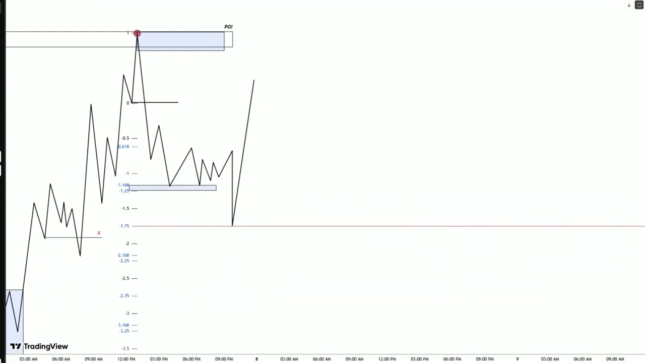
The behavior of price around specific SD levels provides the primary signal for market bias. The most critical levels to monitor are -0.5 and -0.618. These levels act as the gatekeepers for determining whether a high or low is confirmed.
When price approaches a Point of Interest (POI) or a key SD zone, observe the candle closure. If price taps the zone and then closes its body below the -0.5/-0.618 level (in a bearish scenario), the first stage of the bearish narrative is confirmed. This body closure indicates that the market has accepted lower prices and is likely to seek liquidity below. At this point, the probability of price forming a new higher high diminishes significantly.
Following this confirmation, price typically retraces to the -1 to -1.5 zone or the -2 to -2.5 zone. The reaction within these zones determines the depth of the next move.
If price enters the -1/-1.5 zone and moves sideways (consolidates), it signals that the market is not interested in a deep retracement to the extreme POI. Instead, price will likely reject from the First Line of Defense (FLOD) or the nearest internal POI (such as a breaker block or fair value gap) and continue in the direction of the trend. This sideways action is a sign of strength in the immediate direction.
Conversely, if price closes below the -0.5/-0.618 level and then moves sharply without consolidation, it indicates aggressive selling pressure. In this case, price is likely to travel all the way to the Extreme POI. This sharp movement bypasses intermediate support/resistance levels because the algorithm is seeking a deeper liquidity pool or a more significant imbalance. The absence of sideways movement is a key indicator that the extreme level will be tested.
Identifying Hotspots and Sniper Entries▶ 39:00
Within the broader SD zones, specific sub-levels act as Hotspots. These are precise price points where the algorithm reacts with high frequency. Rather than marking entire zones from -2.0 to -2.5, traders should focus on the specific lines within that range, such as -2.168 or -2.25. These hotspots are where limit orders are clustered and where price often reverses with minimal drawdown.
When price reaches a hotspot like -2/-2.5 after a confirmed body closure below -0.618, it presents a low-risk entry opportunity. If price consolidates sideways at this level, it confirms that the extreme POI will not be reached, and the trade can be taken with a tight stop loss above the consolidation range.
However, if price spikes through these levels aggressively, the trader must wait for the reaction at the Extreme POI. The narrative shifts from a shallow retracement to a deep liquidity hunt. Once the Extreme POI is tapped, price often reverses sharply, providing another entry opportunity back towards the -2/-2.5 zones.
The key to sniper entries lies in observing the speed of price arrival. Slow, sideways arrival at -1/-1.5 suggests a rejection from that level. Fast, impulsive arrival suggests a continuation to the extreme. This distinction allows traders to adjust their targets and stop losses dynamically based on real-time price delivery.
Stage-Based Market Narrative▶ 48:00
Market movement unfolds in three distinct stages, each offering different trading opportunities and requiring different analytical focus.
Stage 1: Confirmation and Initial Retracement
This stage begins with the body closure below -0.5/-0.618. The bias is established. Price retraces to -1/-1.5 or -2/-2.5. If sideways movement occurs here, the trade is taken off the FLOD. If sharp movement occurs, the trader waits for the Extreme POI test. The goal in Stage 1 is to capture the initial leg of the true directional move.
Stage 2: Deep Retracement or Continuation
If price reaches the Extreme POI and reverses, it enters Stage 2. Here, price may rally back up to test the breakdown level. If price closes back above the -1/-1.5 zone, the bearish bias is invalidated, and the original high may be taken out. If price rejects from the -2/-2.5 zone again, it confirms the bearish structure, and price will likely fall to -4/-4.5. This stage is crucial for adding to positions or confirming the longer-term trend.
Stage 3: Exhaustion and Reversal
In Stage 3, price reaches the extreme extensions like -4/-4.5. At this point, the market is overextended. Traders look for signs of exhaustion, such as divergence or failure to make new lows. If price consolidates sideways at -4/-4.5, a reversal is imminent. If price spikes through these levels, it may be hunting final stop losses before a major trend change.
Understanding these stages prevents traders from exiting too early or holding losing positions too long. Each stage has a specific set of rules for entry and exit, governed by the interaction between price and SD levels.
Advanced OHLC and IPDA Data Ranges▶ 52:00
To predict market movements accurately, one must understand Advanced OHLC (Open, High, Low, Close) and IPDA Data Ranges. While basic OHLC describes a single candle's profile, Advanced OHLC looks at the relationship between consecutive candles to determine institutional intent.
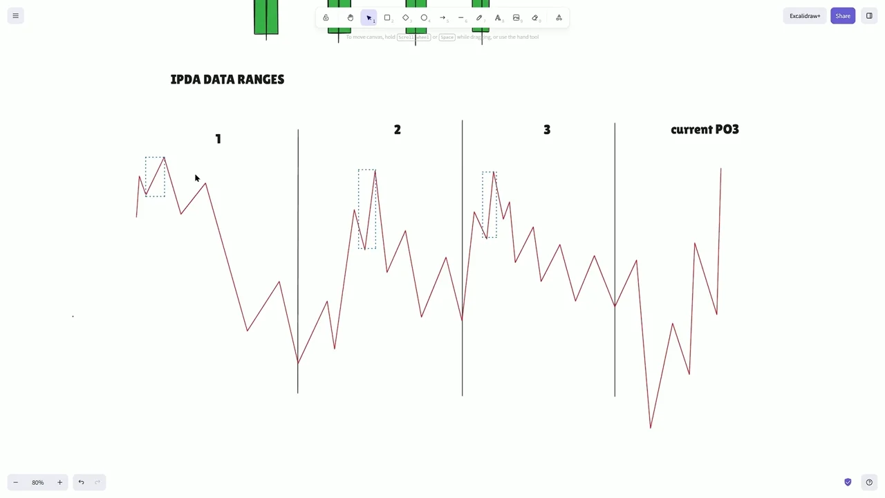
IPDA Data Ranges refer to a lookback period of data used to predict future price delivery. Specifically, the algorithm uses the data from the previous three candles to determine the boundaries and objectives of the current candle. This 3-2-1 rule is fundamental.
By analyzing the highs, lows, opens, and closes of these three prior candles, traders can identify where the current candle is likely to seek liquidity. For instance, if the current Weekly candle opens, it will likely manipulate towards the low of one of the previous three weeks before distributing towards the high of another.
This concept applies across all time frames. For a Daily candle, look at the previous three Daily candles. For a 4-Hour candle, look at the previous three 4-Hour candles. The data from these three candles creates a "range" within which the current candle's manipulation and distribution will occur.
Applying the 3-2-1 Rule to Standard Deviation▶ 61:00
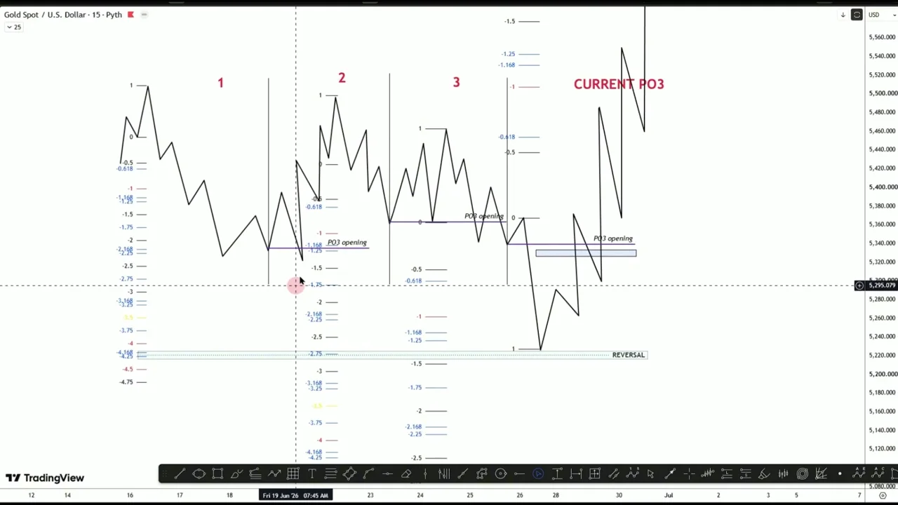
Combining the 3-2-1 IPDA rule with Standard Deviation creates a powerful predictive model. When analyzing the current PO3, plot SD on the manipulation legs of the previous three candles (Candle 1, Candle 2, and Candle 3).
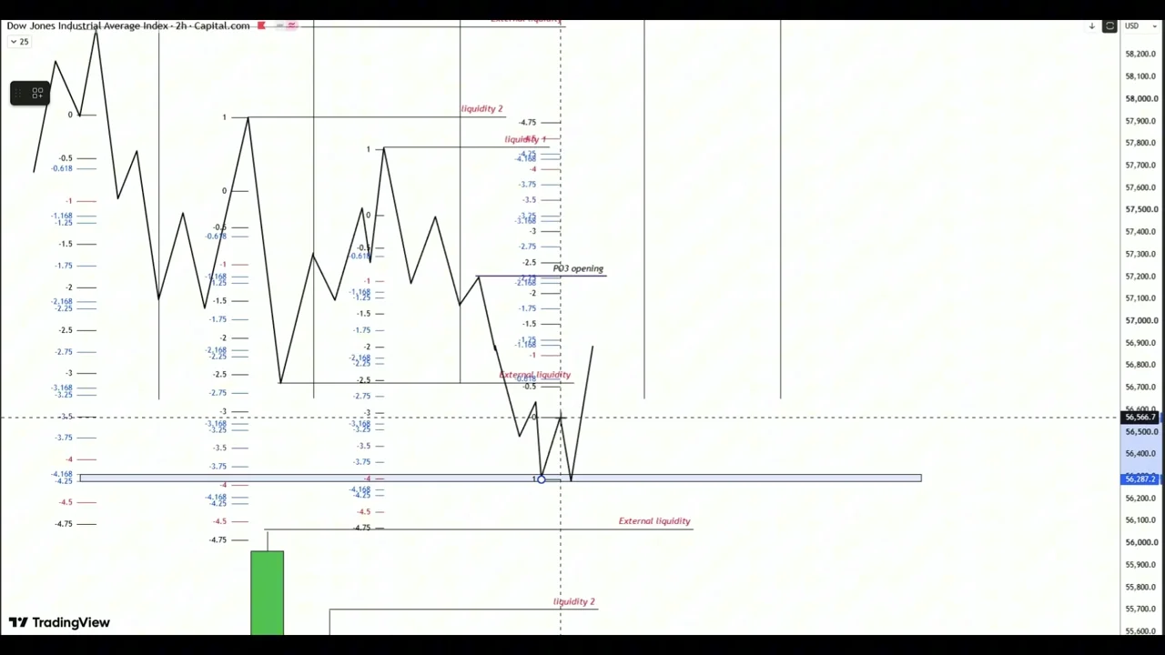
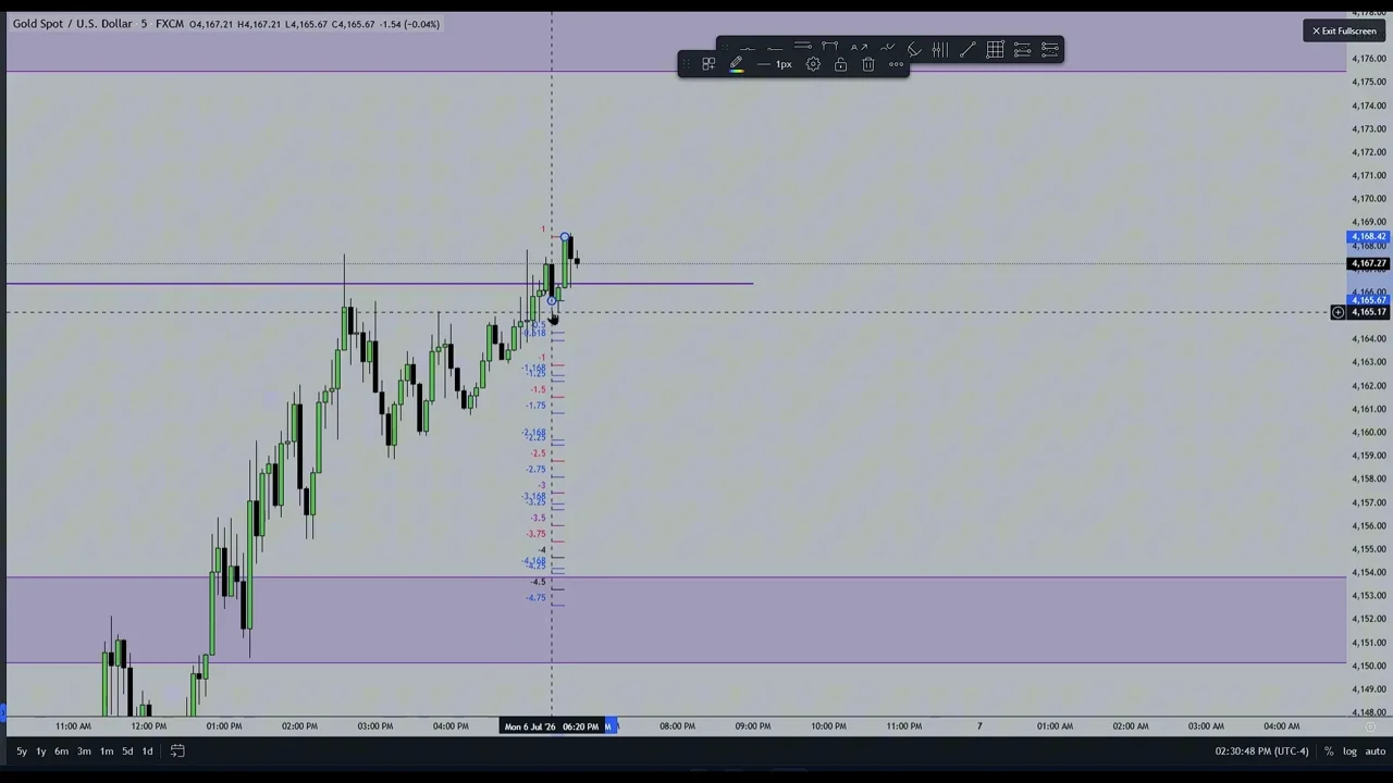
When SD is plotted on the manipulation legs of these three candles, their respective levels (especially the -4/-4.5 extremes and the -1/-1.5 retracement zones) will often align horizontally. These confluence zones are where price is highly likely to reverse.
For example, if the -2.5 level of Candle 1's SD aligns with the -1.5 level of Candle 2's SD and the -4 level of Candle 3's SD, this horizontal cluster becomes a high-probability reversal point. The algorithm is drawing from the data of all three previous candles to execute the current move.
This method removes guesswork. Instead of randomly selecting a swing point, the trader uses the objective data of the last three candles to define the playing field. The "Main Leg" among these three is usually the one with the most significant structure break or liquidity sweep, and its SD levels take precedence.
Practical Example: Gold Weekly Analysis▶ 65:00
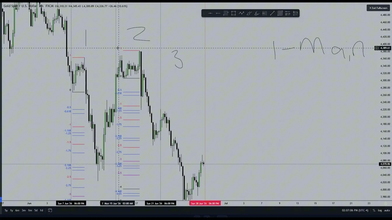
Consider a practical application on the Gold Weekly chart. To trade the current Weekly candle, the trader analyzes the previous three Weekly candles using the 4-Hour and 1-Hour charts for structure (per the time frame alignment rule).
1. Identify the Legs: On the 4-Hour chart, identify the manipulation legs for the previous three weeks.
2. Plot SD: Apply the custom SD settings to these legs.
3. Find Confluence: Observe where the SD levels from Week 1, Week 2, and Week 3 overlap.
4. Mark Liquidity: Identify the external liquidity pools (highs/lows) of the previous three weeks.
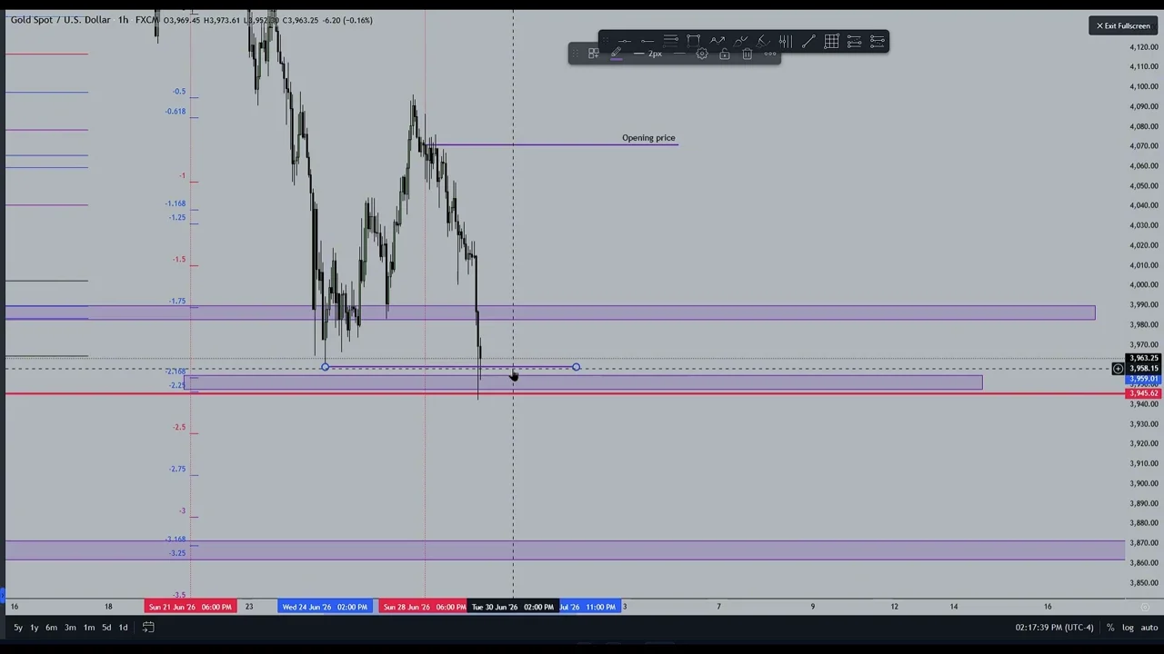
In the example shown, the previous weeks' data indicated a strong confluence zone around a specific price level. When the current Weekly candle opened, it dropped sharply. By monitoring the 1-Hour chart, the trader observed price closing below the -0.618 level of the current week's initial leg. This confirmed the bearish bias.
Price then retraced sideways into the -1/-1.5 zone, rejecting from the First Line of Defense. This sideways action confirmed that the Extreme POI would not be tested immediately. The trader entered a sell position, targeting the -2/-2.5 zones derived from the IPDA data ranges. The price subsequently fell precisely to these targets, validating the framework.
Time-Based Liquidity: The 3-Candle Rule▶ 74:00
A lesser-known but critical concept is Time-Based Liquidity. Most traders understand that price moves from external liquidity to internal liquidity and back. However, they fail to recognize the time constraint imposed on this process.
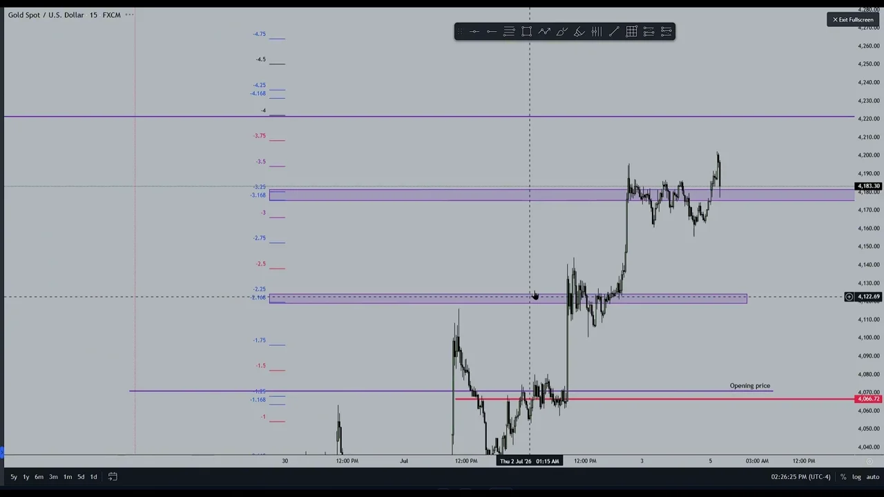
The algorithm operates on a strict timeline. If price hunts an external liquidity pool (e.g., the high of Candle 1), it is expected to seek internal liquidity (e.g., a fair value gap or order block) within the next three candles.
In Scenario B, the failure to respect the 3-candle window indicates that the market is not ready for a deep retracement. Instead, price is likely to seek another external liquidity pool. This is a trend continuation signal, not a reversal signal.
This rule explains why many reversal trades fail. Traders see a liquidity sweep and assume a reversal, ignoring the fact that price has remained near the extreme for more than three candles. The algorithm is signaling that it needs to take out the next external high/low before it can afford to retrace internally.
By counting the candles post-liquidity sweep, traders can filter out low-probability reversals and stay aligned with the dominant trend. If the 3-candle window passes without a significant internal retracement, the bias remains in the direction of the liquidity hunt.
Integrating All Concepts: A Complete Trade Setup▶ 78:00
To execute a trade using this comprehensive framework, follow these steps:
1. Define the Current PO3: Identify the candle you are trading (e.g., Daily, Weekly).
2. Gather IPDA Data: Look at the previous three candles of the same timeframe.
3. Align Time Frames: Drop to the appropriate lower timeframe (e.g., 1-Hour for Daily PO3) to find the manipulation legs of those three previous candles.
4. Plot SD: Apply the custom SD settings to these legs. Identify confluence zones where levels from different candles align.
5. Monitor the Open: Watch the opening of the current PO3 candle.
6. Wait for Confirmation: Observe if price closes its body below/above the -0.5/-0.618 level of the initial move.
7. Assess Speed: Determine if price is moving sharply (indicating an Extreme POI test) or sideways (indicating a shallow retracement).
8. Check Time-Based Liquidity: If a liquidity sweep occurred, count the candles. If >3 candles pass without internal retracement, expect further external liquidity hunting.
9. Enter: Place the trade at the confirmed hotspot (FLOD or Extreme POI) with stops beyond the relevant SD level.
10. Target: Aim for the next SD confluence zone or the opposing external liquidity pool.
This process integrates time, price, and algorithmic data ranges into a single, cohesive narrative. It removes emotional decision-making by providing objective criteria for every step of the trade.
Summary of Key Concepts
By mastering these elements, traders can anticipate market moves with greater precision, distinguishing between noise and genuine algorithmic intent.
AI Perspective
This analysis evaluates key factual claims from the summary, excluding satirical or hyperbolic framing.
| Claim | Verdict | Comment |
|---|---|---|
| Standard Deviation is commonly misrepresented as merely a tool for projecting profit targets. | ✅ Confirmed | SD is widely used for volatility-based targets in retail trading literature. |
| Higher-timeframe candles must be analyzed using specific lower-timeframe structures for SD plotting. | ❓ Unverifiable | A methodological claim within a proprietary system, not an empirically verifiable fact. |
| The market algorithm uses data from the previous three candles to determine the current candle's boundaries. | ❓ Unverifiable | This "3-2-1 rule" is a specific trading heuristic, not a documented market mechanism. |
| A candle body closing below -0.5/-0.618 SD level confirms bearish bias and invalidates a new high. | ❓ Unverifiable | This is a rules-based trading premise; no independent statistical validation is cited. |
| Sideways price movement at -1/-1.5 SD level signals rejection from the "First Line of Defense." | ❓ Unverifiable | This relies on a proprietary framework's internal logic, not a general market fact. |
| If price fails to retrace internally within 3 candles after an external liquidity sweep, it will seek new external liquidity. | ❓ Unverifiable | Presented as an algorithmic rule but lacks external evidence; a backtestable hypothesis. |
| Applying SD to manipulation legs of three prior candles creates high-probability confluence reversal zones. | ❓ Unverifiable | A core premise of the trading strategy, not an independently established fact. |
| Standard SD tools lack timing logic, risking stop-outs during deeper retracements to -2 or -2.5. | ✅ Confirmed | Standard deviation bands alone do not provide timing or trade management signals. |
| Price delivery unfolds in distinct phases: manipulation (stop-hunting) and distribution (value delivery). | ⚠️ Approximate | Aligns with auction market theory but uses ICT-specific terminology without proof of intent. |
| The body closure relative to SD levels is the primary signal for market bias. | ❓ Unverifiable | A rules-based claim within a specific system, not a broadly validated statistical finding. |
इस वीडियो के बारे में पूछें